Gallery

Comparison of the density for different driving parameters

Illustration of a density slice in two MHD turbulence simulations with the same sonic Mach number of approximately 0.5 for the two extreme cases of forcing parameters used our forcing study.

The left panel shows a simulation driven by a delta-in-time (i.e., uncorrelated) acceleration field whose amplitude is normalized to provide a constant (in time) energy injection rate. The right panel shows a simulation driven by an acceleration field governed by a stochastic Ornstein-Uhlenbeck process with an autocorrelation time equal to a dynamical time and constant amplitude.

The time evolution covers five large scale eddy turnover times starting from uniform initial conditions with the fluid at rest. In the stationary regime (after 2.5T) the simulations are subsonic and super-Alfvenic. More information can be found in the corresponding paper.

To download the video use a right-click on the video and select “Save video as”.

Animated illustration of shell decomposition

The video illustrates the shell decomposition we used to study energy transfer between different scales (eddies of different sizes) in compressible MHD turbulence.

Eddies are shown based on the Q-criterion and filtered to indicate regions where the flow is dominated by rotational motion. The top left panel includes information of all spatial scales. The other panels include information of only one individual “shell” with decreasing spatial size from top right, to bottom left, to bottom right.

The time evolution covers five large scale eddy turnover times starting from uniform initial conditions with the fluid at rest. In the stationary regime (after 2.5T) the simulations are subsonic and super-Alfvenic. More information can be found in our corresponding paper.

To download the video use a right-click on the video and select “Save video as”.

Illustration of subgrid-scale modeling

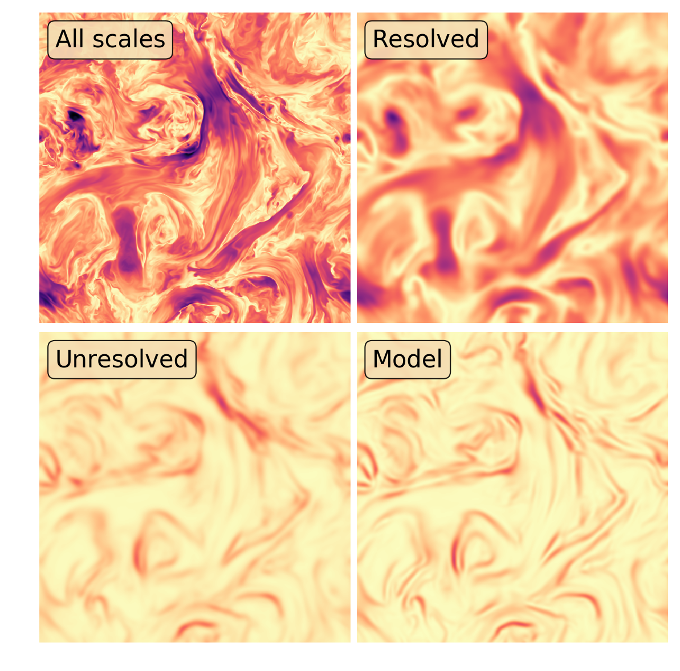
The image displays the magnetic energy in a turbulence simulation. The top left panel shows all relevant scales. Typically only a coarser level of detail can be resolved in a simulation (top right). Effects from the unresolved scales (bottom left) are missing in those simulations. The subgrid-scale model we proposed and verified (see research) is capable to account for those effects and allows to reintroduce them to the simulation.

Illustration of adaptive mesh refinement (AMR)

Traditional hydrodynamic “blast” problem run with AthenaPK on GPUs. An overpressurized region in the center expands over time. The color shows the density and the computational grid/mesh is indicated by the thin black lines.
AthenaPK will implement the (magneto)hydrodynamic methods of Athena++ on top of the performance portable AMR framework Parthenon and Kokkos.

Illustration of the effect of magnetic fields in cloud-crushing/wind-tunnel simulations

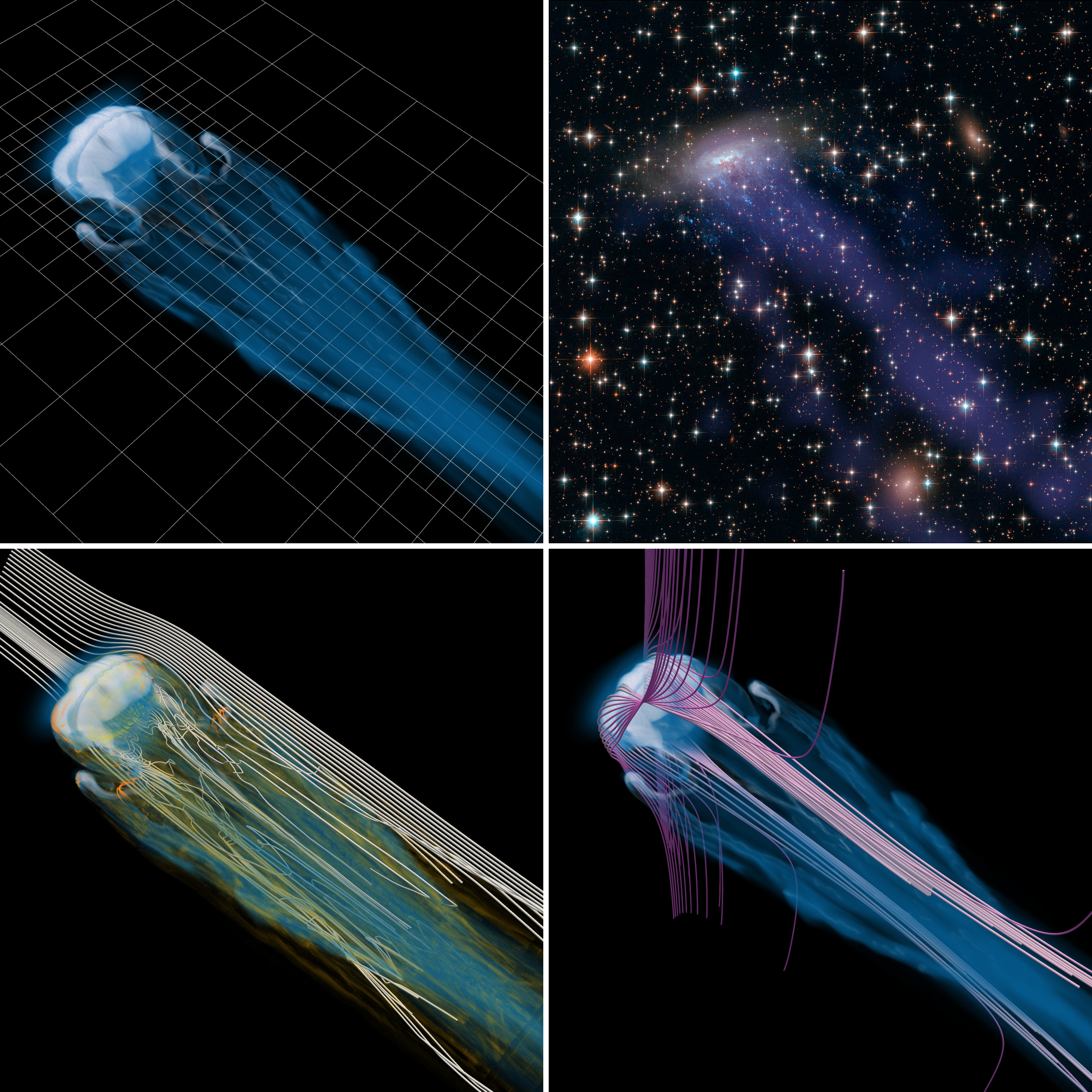
The illustrations shows a volume rendering of the plasma density with the (adaptively refined) simulation grid (top left), velocity streamlines in gray and strong vortical motions in orange (bottom left), magnetic field lines that drape around the cloud (bottom right), and an observation of a “jellyfish” galaxy for reference (top right).

Click image for a high-resolution version.